How To Add Values In Excel Chart

Excel allows us to add or insert desired chart elements such as chart titles legends data labels etc. On the worksheet that contains your chart data in the cells directly next to or below your existing source data for the chart enter the new data.

Chart Tools For Mac Excel 2016 Pro Data Visualization Add In Chart Tool Data Visualization Excel

Select the chart choose the Chart Elements option click the Data Labels arrow and then More Options Uncheck the Value box and check the Value From Cells box.

How to add values in excel chart. Add a data series to a chart on a separate chart sheet. Click the worksheet that contains your chart. To change x axis values to Store we should follow several steps.

Change horizontal axis values. Select the data range that you want to create a chart but exclude the percentage column and then click Insert Insert Column or Bar Chart 2-D Clustered Column Chart see screenshot. To label one data point after clicking the series click that data point.

Add Multiple Columns To A. Pivot Table Basic Sum Exceljet. Click Layout Data Table and select Show Data Table or Show Data Table with Legend Keys option as you need.

Select data for the chart. Select the blank cell beside the first value of the pasted column type the formula COUNTIFA2A24E2 into the cell and then drag the AutoFill Handle to other cells. Click the data series or chart.

In Excel in the Chart Tools group there is a function to add the data table to the chart. 1 Answer1 1 Select cells A2B5 2 Select Insert 3 Select the desired Column type graph 4 Click on the graph to make sure it is selected then select Layout 5. To change the location click the arrow and choose an option.

In the Series name box type the desired name say Target line. Excel Pivot Tables Summarizing Values. How to change x axis values.

Select cells C2C6 to use for the data label range and then click the OK button. Click on the data chart you want to show its data table to show the Chart Tools group in the Ribbon. Chart elements help make our charts easier to read.

Select the source data and click Insert Insert Column or Bar Chart Stacked Column. To insert a chart element we need to click on the Add Chart Element option under the Design tab then. In the Select Data Source dialog box click the Add button in the Legend Entries Series In the Edit Series dialog window do the following.

Right-click the chart and then choose Select. Then all total labels are added to every data point in the stacked column chart immediately. In the formula COUNTIFA2A24E2 A2A24 is the fruit column in source data and E2 is the first unique value in the pasted column.

Select the Edit button and in the Axis label range select the range in the Store column. Pivot Table With Text In Values Area Excel Mrexcel Publishing. Click in the Series value box and select your target values without the column header.

Add Multiple Columns To A Pivot Table Custom. Select Insert Recommended Charts. In the upper right corner next to the chart click Add Chart Element Data Labels.

Select the stacked column chart and click Kutools Charts Chart Tools Add Sum Labels to Chart. The values from these cells are now used for the chart data labels. Select a chart on the Recommended Charts tab to preview the chart.

Select Data on the chart to change axis values. In the Add line to chart dialog please check the Other values option refer the cell containing the specified value or enter the specified value directly and click the Ok button. Add data labels to a chart.

Right-click on the graph and choose Select Data. If you want to. You can select the data you want in the chart and press ALT F1 to create a chart immediately but it might not be the best chart for the data.

How To Add A Column In Pivot Table 14 S With Pictures.

Excel Charts Multiple Series And Named Ranges Chart Name Activities Create A Chart

Pin On Business Industrial

Excel Chart Of Top Bottom N Values Using Rank Function And Form Controls Pakaccountants Com Excel Tutorials Data Dashboard Excel Shortcuts

Target Vs Actual Charts Excel 4 Thermometer Charts Chart Excel Tutorials Microsoft Excel Formulas

How To Create A 2d Clustered Column Chart In Microsoft Excel Microsoft Excel Chart Excel

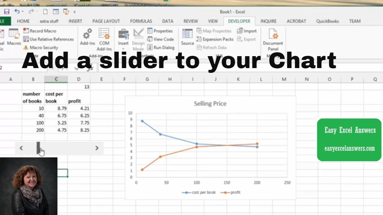
Add A Slider To Your Chart In Excel Excel Excel Shortcuts Job Information

How To Reverse Order Of Chart In Excel Chart Excel Reverse

Moving X Axis Labels At The Bottom Of The Chart Below Negative Values In Excel Pakaccountants Com Excel Tutorials Excel Excel Shortcuts

Excel Magic Trick 267 Percentage Change Formula Chart Youtube Microsoft Excel Tutorial Formula Chart Excel Tutorials

Excel Variance Charts Making Awesome Actual Vs Target Or Budget Graphs How To Pakaccountants Com Excel Tutorials Excel Shortcuts Excel

Add Vertical Date Line Excel Chart Myexcelonline Line Scroll Bar Excel

Making A Slope Chart Or Bump Chart In Excel How To Pakaccountants Com Microsoft Excel Tutorial Excel Tutorials Excel

Create Excel Waterfall Chart Excel Tutorials Excel Spreadsheet Design

Pin On Microsoft Products

Excel Charts Microsoft Excel Computer Lab Lessons Excel

8 Free Excel Add Ins To Make Visually Pleasing Spreadsheets Charts And Graphs Excel Spreadsheet

Create A Simple Bar Chart In Excel 2010 Excel Spreadsheets Bar Chart Charts And Graphs

A Typical Column Chart Containing A Variety Of Standard Chart Elements Excel Computer Lab Lessons Instructional Design

How To Create Graphs In Excel Create Graph Graphing Excel