How To Add Two Sets Of Data To An Excel Graph

12 Jun, 2021

To create a combo chart select the data you want displayed then click the dialog launcher in the corner of the Charts group on the Insert tab to open the Insert Chart dialog box. Insert the data in the cells.

Using Error Bars For Multiple Width Chart Series Bars Chart Data Visualization Column

This plot will look like.

How to add two sets of data to an excel graph. Leaving the dialog box open click in the worksheet and then click and drag to select all the data you want to use for the chart including the new data. To create a chart select your data set and click Insert Recommended Charts or click a chart that you want. Select combo from the All Charts tab.

Create the Time Series A line chart above left copy the Time Series B data select the chart and use Paste Special to add the data as a new series using the options as shown. As before click Add and the Edit Series dialog pops up. For var i 0.

Once this is done click OK and you now have your completed chart. From the pop-down menu select. In the combination chart click the line chart and right click or double click then choose Format Data Series from the text menu see screenshot.

But if you are worried about the spread of data in set 1 and set 2 and difficulty in pattern understanding you can switch x y and you can use secondary axis. The Select Data Source dialog box appears on the worksheet that contains the source data for the chart. Select Series Data.

I internaldatalength 27 in this example if i 0 i 14 countrypushinternaldatai0. Right-click the chart and choose Select Data. Select the Secondary Axis box for the data you want to move to the secondary.

To merge two sets of data into one graph in Excel select both sets of data that will comprise the graph. Click Add above the bottom-left window to add a new series. Now click on Insert Tab from the top of the Excel window and then select Insert Line or Area Chart.

Fill in entries for series name and Y values and the chart shows two series. After insertion select the rows and columns by dragging the cursor. If you have created a column chart you can select the item Data Edit data in the function bar and thus add a second data series.

Follow the below steps to implement the same. Time series A has weekly data but with two values omitted. Months dataApush parseIntinternaldatai1 value 2015 countryA parseIntinternaldatai2 value 2016 countryA parseIntinternaldatai3 value 2017 countryA.

Goto Design tab and Select Data Add the new series and select data points in new series. In the Edit Series window click in the first box then click the header for column D. Now you can select the Line display under Type under the function bar via Colors and Style.

If i 13 i 27 dataBpush parseIntinternaldata. The two data series. Right-click the chart and then choose Select Data.

Right click the chart and choose Select Data from the pop-up menu or click Select Data on the ribbon. Now our aim is to plot these two data in the same chart with different y-axis. There are spaces for series name and Y values.

This time Excel wont know the X values automatically. Choose the type of chart you want to use for each data set in the table at the bottom of the Insert Chart dialog. Select the chart type you want for each data.

Next choose an option called Combo from the parent group titled All Charts A benefit of using Microsoft Excel as a spreadsheet application is that it displays simple information just as clearly as it does more complex graphs. Hope you wanted either of this. Time series B has more data points at irregular intervals over a shorter time span.

In order to add two trend lines youll need to have data for more than one thing like the performance of two or more sales people instead of. To do this right click on the chart and then click select data and then rename the legend entries by clicking on the first legend entry and inputting 2017 into the Name field and then doing the same for the 2 nd. And it will look like.

If i 0. In the Format Data Series dialog click Series Options option and check Secondary Axis see screenshot.

Directly Labeling In Excel Evergreen Data Line Graphs Labels Data

Excel Charts Multiple Series And Named Ranges Chart Name Activities Create A Chart

How To Create A Double Lollipop Chart Chart Chart Tool Lollipop

How To Plot Multiple Data Sets On The Same Chart In Excel 2010 Excel Chart Design Chart

Super Helpful Description Of How To Graph Two Y Axes In Excel Graphing Excel Chart

Multiple Time Series In An Excel Chart Peltier Tech Blog Time Series Chart Excel

World Polls Chart Very Nicely Done Chart To Combine Multiple Data Sets Free Excel Chart Template Download T Radar Chart Charts And Graphs Pie Chart Template

Changing The Default Chart Type In Excel Chart Bar Graph Template Graphing

Adding A Benchmark Line To A Graph Evergreen Data Performance Measurement Data Visualization Benchmark

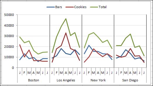
How To Create A Panel Chart In Excel Excel Shortcuts Chart Excel Tutorials

Excel Variance Charts Making Awesome Actual Vs Target Or Budget Graphs How To Pakaccountants Com Excel Tutorials Excel Shortcuts Excel

5 Steps To Making Formatting A Line Graph In Excel Line Graphs Graphing Excel

Add A Slider To Your Chart In Excel Excel Excel Shortcuts Job Information

Try Using A Line Chart In Microsoft Excel To Visualize Trends In Your Data Excel Microsoft Excel Tutorial Line Chart

How To Create Graphs In Excel Create Graph Graphing Excel

07 Combo Chart Set Number To Currency And Decimal Point Chart Combo Text

Side By Side Bar Chart Combined With Line Chart Welcome To Vizartpandey Bar Chart Line Chart Chart

Graphing Multiple Baseline Design Applied Behavior Analysis Behavior Analysis Graphing