How To Put Numbers On Excel Graph
In a chart click the value axis that you want to change or do the following to select the axis from a list of chart elements. Select the source data and click Insert Insert Column or Bar Chart Stacked Column.
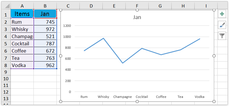
How To Add A Single Data Point In An Excel Line Chart
How do you add footnotes in Excel.

How to put numbers on excel graph. For example ROW A1 returns the number 1. The Scale tab provides different options for a category x axis. Assuming youre using Excel 2007 data labels are added through the Data Labels selection.
If your chart has labels Right click on the label. In the Series name box type the desired name say Target line. These are the steps to achieve the result.
Click Add button to apply number format. When you hit Enter the chart title will display what ever is in the cell with your formula and will dynamically change as you change the selected year. Once your data is selected click Insert Insert Column or Bar Chart.
You can do this manually using your mouse or you can select a cell in your range and press CtrlA to select the data automatically. To insert a bar chart in Microsoft Excel open your Excel workbook and select your data. Use the ROW function to number rows.
Click anywhere in the chart. Choose Format Data labels. Select the range A1D7.
You can also double-click the chart to launch the Format Object Task Pane which will appear on the right-hand side of the Excel windowThis will also expose the map chart specific Series options see below. Go to Custom and key in 0 K in the place where it says General and close the popup. On the Number format Choose Custom from the drop down.
Formatting your Map chart. Only if you have numeric labels empty cell A1 before you create the line chart. This video shows y.
Next click into the chart title on your chart then go to the Formula Bar and type in an equal sign and the location where you put the previous formula. You can also choose Number Formatting from the Home Ribbon or simply press the shortcut Ctrl 1. As shown below cells A2A5 contain the data Items.
Go to the Number tab in the Format Cells menu. 2 Select Insert 3 Select the desired Column type graph. Drag the fill handle across the range that you want to fill.
Simply select the number cell or a range of numbers that you would like to simplify. Select a preset number format or Custom in Category dropdown. You can also access the Format Cells menu using the Ctrl 1 keyboard shortcut.
I wanted labels in millions as it is space wise more economical. Click Line with Markers. The important point here is that a number format can be applied.
On the Insert tab in the Charts group click the Line symbol. If are using Excel 2010 it will open the Format Axis. The ROW function returns the number of the row that you reference.
In the Format Axis pane please expand the Number section type the custom format code in the Format Code box and click the Add button. Then add a chart title to your chart. Just click on the map then choose from the Chart Design or Format tabs in the ribbon.
4 Click on the graph to make sure it is selected then select Layout. To change the interval of tick marks and chart gridlines type a different number. Right click and select Format Cells from the menu.
Then all total labels are added to every data point in the stacked column chart immediately. Cells B2B5 contain the data Values. Right-click the existing graph and choose Select Data from the context menu.
Often a table or chart in a financial report requires a footnote to give full disclosure to the viewer. Type your custom number format code into Format Code textbox. Select the data from your table where you want add symbols.
To change the number at which the value axis starts or ends type a different number in the Minimum box or the Maximum box. 1 Select cells A2B5. In Excel you can apply any number format on value-axis values as you can apply them to cells that contains numbers.
On the Format tab in the Current Selection group click the arrow next to the Chart Elements box and then click Vertical Value Axis. In the first cell of the range that you want to number type ROW A1. Once your map chart has been created you can easily adjust its design.
Expand NUMBER section. In the Select Data Source dialog box click the Add button in the Legend Entries Series In the Edit Series dialog window do the following. Right Click and choose Custom Formatting.
Select the stacked column chart and click Kutools Charts Chart Tools Add Sum Labels to Chart. For example to show the date as 314 I type md in the Format Code box.

How To Add A Day To A Schedule In Excel Excel Day Ads

Chart Tip Kiss Chart Excel Bar Chart

How To Move Chart X Axis Below Negative Values Zero Bottom In Excel

How Do You Put Values Over A Simple Bar Chart In Excel Cross Validated
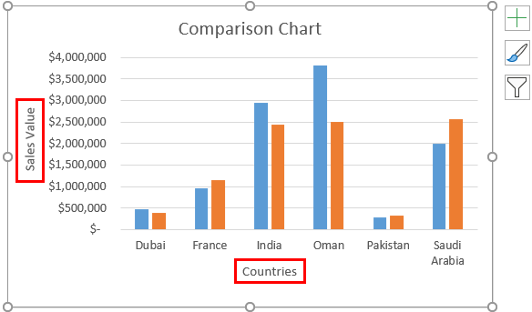
Comparison Chart In Excel Adding Multiple Series Under Same Graph

How To Create A Chart By Count Of Values In Excel

How To Change Axis Values In Excel Excelchat
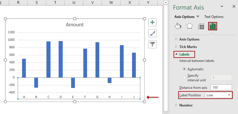
How To Move Chart X Axis Below Negative Values Zero Bottom In Excel

Pin On Software
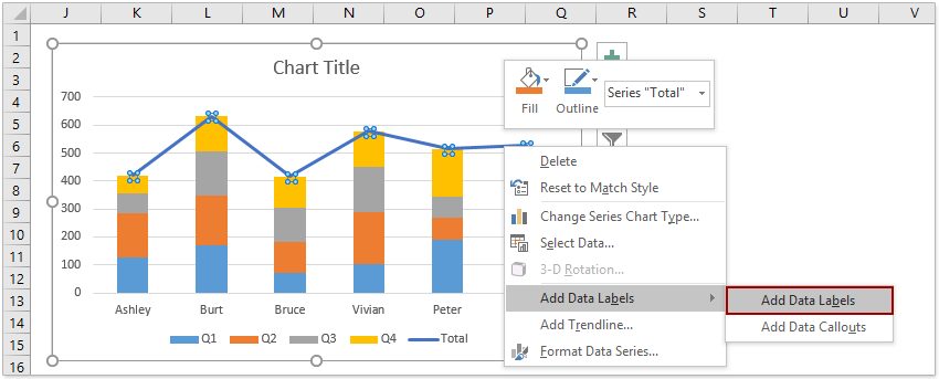
How To Add Total Labels To Stacked Column Chart In Excel
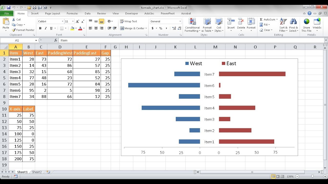
Create A Tornado Butterfly Chart Excel Shortcuts Excel Diagram

Excel Charts Add Title Customize Chart Axis Legend And Data Labels

How To Add A Right Hand Side Y Axis To An Excel Chart

Here S How To Use Excel Shortcuts To Quickly Add Worksheets Excel Shortcuts Excel Worksheets

How To Add Secondary Axis In Excel In 2021 Excel Secondary Axis

How To Change Number Format In Excel Chart
Group Data In An Excel Pivottable Pivot Table Excel Data
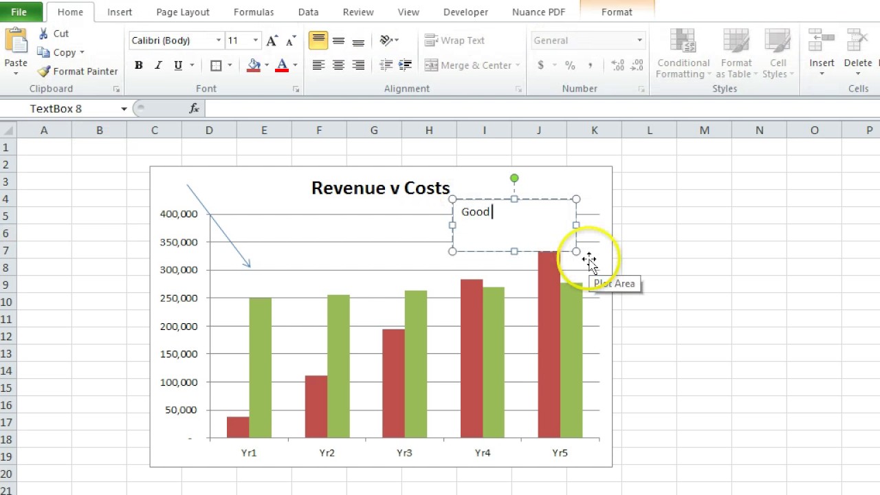
How To Add Text Boxes And Arrows To An Excel Chart Youtube

How To Make A Graph In Excel A Step By Step Detailed Tutorial