How To Add Multiple Rows In Excel Pivot Table

Click and drag a field to the Rows. The pivot table rows should be now placed next to each other.

Multi Level Pivot Table In Excel Pivot Table Excel Microsoft Excel

Multiple fields as row labels on the same level in pivot table Excel 2016.

How to add multiple rows in excel pivot table. Preventing nested grouping when adding rows to pivot table in Excel. In the INSERT menu select the Pivot Table. This can be done easily by adding a subtotal to the pivot table.

Now lets create a pivot table Insert Tables Pivot Table and check all the values in Pivot Table Fields. Click a blank cell that is not part of a PivotTable in the workbook. After creating the pivot table firstly you should add the row label fields as your need and leaving the value fields in the Choose fields to add to report list see screenshot p 2.

The range field will be filled in automatically since we have set the cursor in the data cell. Below are the steps to create pivot table from multiple sheets Click AltD then click P. Hold down the ALT F11 keys to open the Microsoft Visual Basic for Applications window.

The table is going to change. Right-click the field name and then select the appropriate command Add to Report Filter Add to Column Label Add to Row Label or Add to Values to place the field in a specific area of the layout section. Now the pivot table should look like this.

Otherwise pick one or two then click Select Related Tables to auto-select tables that are related to those you selected. Press Enter and in the Select Database and Table box choose the database you want then click Enable selection of multiple tables. This function also lets you drag and drop field settings within your pivot t.

Right-click inside a pivot table and choose PivotTable Options. Consolidate multiple worksheets into one PivotTable - Excel. Fields should look like this.

Follow the steps to know how to create multiple subtotals in pivot table. You can also turn off the Classic PivotTable. Click Insert Module and paste the following code in the Module Window.

Click the column label selected drag and drop it into the Row Labels section of the Pivot Table Field List. The Create Table dialog box opens. How to use Excels Classic view to have multiple rows to filter in a pivot table.

By arranging the heads in the pivot table fields by dragging them as per the requirement the data will be projected as given in the image. I have data that lists product models along with relevant data and also production volumes by month. Pivot Tables have a clever feature that allows you to drag multiple rows and columns to the same Pivot Table to add a whole new level of flexibility to your.

Excel will detect the size of the dataset and will suggest to place the pivot table into a new sheet. On Step 1 page of the wizard click Multiple consolidation ranges and then click Next. Click any cell in the PivotTable.

Click any one cell in the pivot table and right click to choose PivotTable Options see screenshot. In that dialogue box select Multiple consolidation ranges and click NEXT. As a next step you have to modify the Field settings of the rows.

Part of the relevant data are about 5 common part columns with the part that applies to each model under the appropriate column. Select the order for the row labels that best suits your needs. I am using Excel 2016.

Check data as shown on the image below. Then swich to Display tab and turn on Classic PivotTable layout. The PivotTable Fields pane appears.

In subtotals section choose None. Make row labels on same line with PivotTable Options. Currently however when I add age and gender to the row category of pivot tables it forms a nested group by.

On Step 2a page of the wizard click Create a single. Select on any cell in the first block of data and click Insert Table or press Ctrl T. The following dialogue box will appear.

Instead I need to have un-nesteddistinct. Click and hold a field name and then drag the field between the. To know how to create a Pivot table please Click Here.

In the list select PivotTable and PivotChart Wizard click Add and then click OK. The Create PivotTable menu opens where we select the range and specify the location. You can also turn on the PivotTable Fields pane by clicking the Field List button on the Analyze tab.

If the cursor is in an empty cell you need to set the range manually. The first step is to create a pivot table for the data. With the picture above in mind I am trying to form pivots for each different age category and gender using Excel 2016.

In the PivotTable Options dialog box click the Display tab and then check Classic PivotTable layout enables dragging of fields in the. You have to right-click on pivot table and choose the PivotTable options. Add an Additional Row or Column Field.

Check the range encompasses all the data and ensure my data has headers is ticked. Click OK Once the pivot table sheet is created just like in the previous example drag the Category and the Product to the Rows section and the Sales Value to the Values section to get the same Multi-Row pivot table we did in the previous example. Reorder the field labels in the Row Labels section and note the changes made to the pivot table.

If you know exactly which tables you want to work with manually choose them.

Excel Vba Macros Sql Examples Tutorials Free Downloads How To Sort Pivot Table Row Labels Column Field L Excel Pivot Table Sorting

Excel Vba Macros Sql Examples Tutorials Free Downloads How To Set The Pivot Table Grand Totals On For Row Pivot Table Excel Microsoft Excel

Multi Level Pivot Table In Excel Pivot Table Excel Excel Templates

Sorting In Pivot Table Select One Of The Values You Wish To Sort Select The Options Tab In Sort Group Click On Way P Pivot Table Excel Tutorials Sorting

Follow These Easy Steps To Create A Pivot Table In Microsoft Excel 2016 Excel Pivot Table Microsoft Excel Tutorial

50 Things You Can Do With Excel Pivot Table Myexcelonline Excel Tutorials Pivot Table Excel

Pivot Table In Excel Pivot Table Excel Pictures Online

Connect Slicers To Multiple Excel Pivot Tables Myexcelonline Pivot Table Microsoft Excel Tutorial Excel Tutorials

Connect Slicers To Multiple Excel Pivot Tables Myexcelonline Excel Tutorials Pivot Table Microsoft Excel Tutorial

Multi Row And Multi Column Pivot Table Pivot Table Excel Tutorials Column

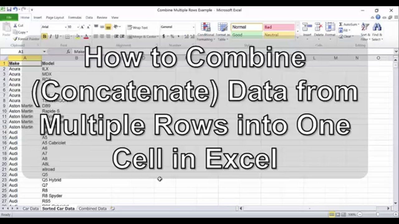
Combine Concatenate Multiple Rows Into One Cell In Excel Excel Excel Hacks Cell

Excel Pivot Tables Pivot Table Excel Tutorials Excel

23 Things You Should Know About Excel Pivot Tables Pivot Table Excel Pivot Table Excel

Multi Level Pivot Table In Excel Pivot Table Excel Microsoft Excel

Connect Slicers To Multiple Excel Pivot Tables Myexcelonline Excel Tutorials Microsoft Excel Tutorial Pivot Table

How To Generate Multiple Reports From One Pivot Table Excel Excel Formula Overlays

How To Insert A Blank Row In Excel Pivot Table Myexcelonline Pivot Table Excel Tutorials Excel

Convert Pivot Table To Sumifs Formulas Free Vba Macro Pivot Table Formula Excel Formula

Making Budget Vs Actual Profit Loss Report Using Excel Pivot Tables Budgeting Excel Excel For Beginners